Normality Test Explained: Types, Methods, Examples

Getting your Trinity Audio player ready...

Contents

• What Is Normal Distribution?
• Methods of Assessing Normality
• How Sample Size Affects Normality Testing
• What to Do When Data Is Not Normally Distributed
• How to Run Normality Tests: Step-by-Step Examples by Software
• Normality Assumption in Regression Analysis
• Frequently Asked Questions About Normality Testing
• Key Takeaways

A normality test is a statistical procedure that determines whether a set of sample data has been drawn from a normally distributed population. Running this test is one of the most important (and most frequently overlooked) steps before performing any parametric statistical analysis.

Most widely used statistical procedures, including t-tests, ANOVA, Pearson correlation, and linear regression, assume that the data (or the residuals of the model) follow a normal distribution. When this assumption is violated and ignored, the results can be entirely misleading: truly significant findings may appear non-significant, or non-significant findings may appear significant.

This guide covers:

• What normal distribution is and why it matters
• Graphical methods for assessing normality
• Statistical tests for normality, with a comparison of five major tests
• How to interpret p-values from normality tests
• What to do when data is not normally distributed
• How to run normality tests in R, Python, SPSS, and Excel
• How sample size affects normality testing

What Is Normal Distribution?

Normal distribution, also known as Gaussian distribution, is the most important probability distribution for continuous, independent random variables in statistics. Most researchers recognize it as the familiar bell-shaped curve seen in statistical reports.

Key Properties of a Normal Distribution

• Symmetric about the mean: the right side is a mirror image of the left side
• Mean, median, and mode are all equal and located at the center (peak) of the curve
• Data near the mean occurs more frequently than data at the extremes (tails)
• The total area under the curve equals 1, representing 100% probability
• Approximately 68% of data falls within 1 standard deviation of the mean, 95% within 2, and 99.7% within 3 (the empirical rule)

Normal distributions apply specifically to continuous variables. Discrete count data and proportional data often require different approaches (see the section on transformations below).

Why Normal Distribution Matters in Research

Parametric statistical tests are built on the mathematical properties of the normal distribution. When these properties hold, parametric tests are the most statistically powerful choice as they are more likely to detect a true effect when one exists. When these properties are violated, parametric tests can produce unreliable p-values, inflated Type I error rates, or misleading confidence intervals.

Methods of Assessing Normality

There are two broad categories of methods for assessing whether data follow a normal distribution: graphical methods and statistical (analytical) tests. Best practice is to use both together, especially for publication.

Graphical Methods

Graphical methods provide an intuitive, visual assessment of normality. They are especially useful during exploratory data analysis and are always recommended as a first step before running formal tests.

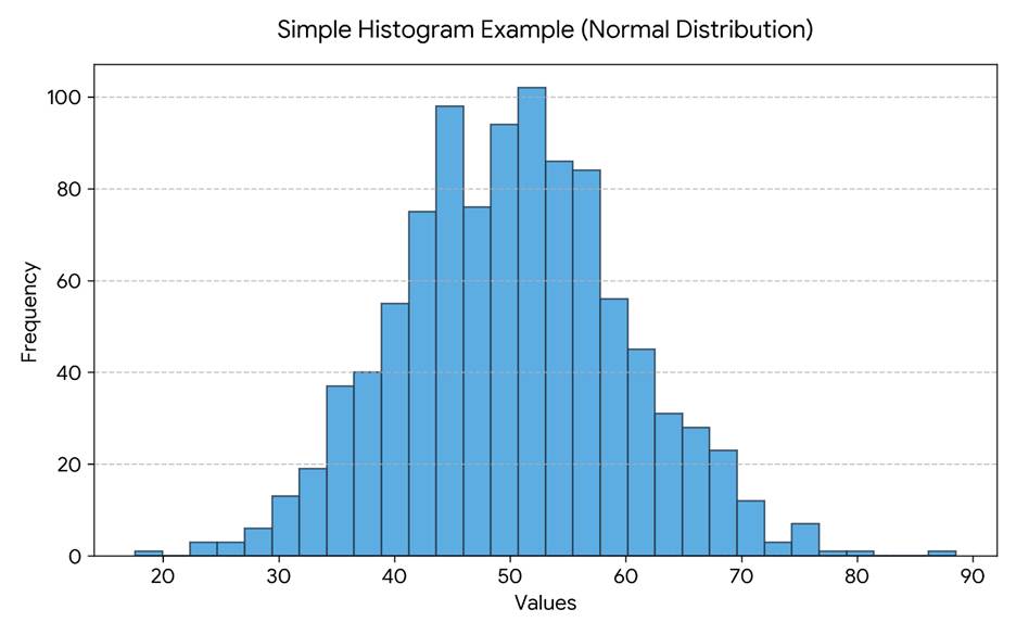
Histogram

A histogram plots the frequency distribution of a variable. For normally distributed data, the histogram should show a roughly symmetric, bell-shaped pattern with a single peak at the center and tails tapering off on both sides. Histograms are less reliable for small sample sizes (n < 20) because random variation can make normal data appear skewed.

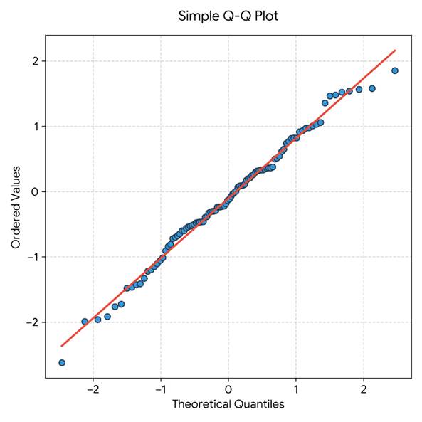
Q-Q Plot (Quantile-Quantile Plot)

A Q-Q plot compares the quantiles of the observed data to the quantiles of a theoretical normal distribution. If the data are normally distributed, the points on the Q-Q plot will fall approximately along a straight diagonal reference line.

How to read a Q-Q plot:

• Points tightly along the diagonal line: data are approximately normal
• Points curving upward at both ends (S-shape): heavy tails (leptokurtosis)
• Points curving below the line at the left and above at the right: right skew (positive skew)
• Points curving above the line at the left and below at the right: left skew (negative skew)

Q-Q plots are generally more informative than histograms for detecting subtle departures from normality, especially in moderate to large samples.

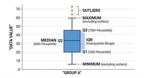
Box Plot

A box plot (or box-and-whisker plot) provides a quick visual summary of the data’s distribution. For normally distributed data:

• The median line should be roughly centered within the box
• The box (interquartile range) should be roughly symmetric
• Whiskers should be approximately equal in length
• Outliers (points beyond the whiskers) should be rare

Statistical (Analytical) Tests for Normality

Statistical tests for normality quantify how much the observed data deviate from a theoretical normal distribution, and express this as a p-value. If the p-value is less than the chosen significance level (commonly 0.05), the null hypothesis of normality is rejected.

Interpreting the p-value

• p ≥ 0.05: No significant evidence of non-normality; proceed with parametric tests
• p < 0.05: Data significantly deviate from normal distribution; consider non-parametric tests or data transformation

Important caveat: With very large samples (n > 200), even trivially small and practically unimportant departures from normality will produce p < 0.05. Always pair the p-value with a visual assessment and consider the practical size of the deviation.

Comparison of the Five Major Normality Tests

The table below summarizes the most commonly used normality tests, including their optimal use cases and key differences:

Test	Best Sample Size	What It Measures	Strengths	Limitations	Typical Use
Shapiro-Wilk	n < 50 (optimal); up to 2,000	Correlation between data and normal scores	Most powerful for small samples	Less reliable for n > 2,000	Small-sample biomedical, clinical research
Kolmogorov-Smirnov (K-S)	n > 50	Max difference between observed and theoretical CDFs	Works for large samples; less sensitive to outliers	Low power for small samples	Quality control, large datasets
D’Agostino-Pearson	n ≥ 20	Skewness and kurtosis combined	Detects skew and heavy tails separately	Requires at least 20 observations	General-purpose normality testing
Anderson-Darling	n ≥ 8	Weighted deviations in distribution tails	More sensitive to tail departures	Less commonly reported in social sciences	Engineering, reliability testing
Lilliefors (Modified K-S)	n > 30	K-S adjusted for estimated parameters	Better than K-S when mean/SD are unknown	Less powerful than Shapiro-Wilk	When population parameters are unknown

Which Test Should You Use?

Use the following as a practical guide:

Sample Size	Recommended Test	Reason
n < 50	Shapiro-Wilk	Most statistically powerful for small samples
n = 50–200	Shapiro-Wilk or D’Agostino-Pearson	Both perform well; D’Agostino-Pearson also detects skew and kurtosis separately
n > 200	Graphical methods (Q-Q plot, histogram)	Formal tests flag trivial deviations as significant; visual inspection is more meaningful
Proportions or unknown population parameters	Lilliefors (modified K-S)	Adjusted for situations where mean and SD are estimated from the data
Engineering or reliability testing	Anderson-Darling	More sensitive to tail departures, which matter most in these contexts
General-purpose, any size	D’Agostino-Pearson	Combines skewness and kurtosis; widely applicable across disciplines

How Sample Size Affects Normality Testing

Sample size has a profound effect on the outcome of normality tests, and this is one of the most misunderstood aspects of statistical practice.

Small Samples (n < 30)

• Normality tests have low statistical power. They may fail to detect non-normality even when it exists
• Graphical methods are unreliable due to random variation
• By convention, parametric tests are sometimes still used with small samples when there is no strong theoretical reason to expect non-normality

Moderate Samples (n = 30–200)

• Normality tests perform optimally in this range
• The Central Limit Theorem begins to apply: the sampling distribution of the mean approaches normality regardless of the underlying distribution
• Both graphical and statistical methods are informative

Large Samples (n > 200)

• Formal normality tests almost always return p < 0.05 due to their high statistical power
• This does not necessarily mean that the deviation from normality is practically important
• Use visual inspection (Q-Q plots, histograms) and effect size measures (skewness, kurtosis) to judge whether the departure matters

Rule of thumb: For large samples, if the skewness value is between -1 and +1 and kurtosis is between -2 and +2, the data are often considered sufficiently normal for parametric analysis.

What to Do When Data Is Not Normally Distributed

When data fail normality tests, there are two broad strategies: switch to non-parametric tests, or transform the data to achieve approximate normality.

Strategy 1: Use Non-Parametric Tests

Non-parametric tests make no assumption about the distribution of the data. They are appropriate when:

• Sample sizes are small and non-normality is detected
• Data are ordinal or ranked
• The distribution is severely skewed and transformation is not feasible

The table below lists the parametric test and its non-parametric equivalent for common scenarios:

Scenario	Parametric Test	Non-Parametric Equivalent	Notes
Compare 2 independent groups	Independent t-test	Mann-Whitney U test	Check normality in each group separately
Compare 2 paired/related groups	Paired t-test	Wilcoxon Signed-Rank test	Used for before/after designs
Compare 3+ independent groups	One-way ANOVA	Kruskal-Wallis test	Post-hoc tests differ by approach
Measure association	Pearson correlation	Spearman rank correlation	Spearman also handles monotonic non-linear relationships
Predict outcome from predictors	Linear regression	Log-rank, quantile regression (context-dependent)	Residuals, not raw data, must be normally distributed

Non-parametric tests are generally less statistically powerful than parametric tests when the normality assumption is actually met. Use them when the assumption is genuinely violated, not as a default to avoid checking.

Strategy 2: Transform the Data

Data transformation applies a mathematical function to each value to reduce skewness and bring the distribution closer to normality. After transforming, re-run the normality test to confirm improvement. Remember to back-transform results when reporting findings in the original scale.

Transformation	When to Use	Formula	Example Use Case
Log transformation	Right-skewed data (positive skew)	log(x) or log(x+1) if zeros present	Income, microbial counts, enzyme levels
Square root	Moderately right-skewed; count data	√x or √(x+0.5)	Counts of events, ecological data
Reciprocal (inverse)	Severely right-skewed data	1/x	Reaction times, survival times
Box-Cox	When optimal transformation is unknown	Automatic lambda estimation	General-purpose; available in R, Python, SPSS
Arcsine (angular)	Proportions or percentages	arcsin(√x)	Proportional data, gene expression frequencies

After transforming, always re-check normality with both a graphical method and a formal test. Report that a transformation was applied and specify which one in the Methods section of your paper.

How to Run Normality Tests: Step-by-Step Examples by Software

Shapiro-Wilk Test in R

R is the most widely used environment for statistical analysis in academic research. The built-in shapiro.test() function runs the Shapiro-Wilk test.

# Run Shapiro-Wilk test

shapiro.test(your_variable)

# Q-Q plot

qqnorm(your_variable)

qqline(your_variable)

Interpretation:

Look for W (the test statistic) close to 1.0 and p > 0.05 for normality. The nortest package also provides the Anderson-Darling test (ad.test()) and Lilliefors test (lillie.test()).

Normality Test in Python

Python’s scipy.stats module provides several normality tests.

from scipy import stats

import matplotlib.pyplot as plt

# Shapiro-Wilk test

stat, p = stats.shapiro(your_data)

# D’Agostino-Pearson test

stat, p = stats.normaltest(your_data)

# Q-Q plot

stats.probplot(your_data, plot=plt); plt.show()

Normality Test in SPSS

SPSS is widely used in social science and medical research. To run normality tests:

1. Go to Analyze > Descriptive Statistics > Explore
2. Move your variable(s) to the Dependent List box
3. Click Plots and check Normality plots with tests
4. Click Continue, then OK

SPSS will output both the Shapiro-Wilk test and the Kolmogorov-Smirnov (Lilliefors-corrected) test, along with a Q-Q plot and histogram. For samples smaller than 50, rely on the Shapiro-Wilk result.

Normality Test in Excel

Excel does not include a built-in normality test, but you can check normality using descriptive statistics and a histogram:

1. Install the Analysis ToolPak add-in (File > Options > Add-ins > Analysis ToolPak)
2. Go to Data > Data Analysis > Histogram to plot the distribution
3. Calculate skewness using =SKEW(range) and kurtosis using =KURT(range)
4. Create a Q-Q plot manually by ranking data and plotting against theoretical normal quantiles

For formal normality testing in Excel, consider using a dedicated statistics add-in such as XLSTAT, which provides Shapiro-Wilk, Anderson-Darling, and other tests natively.

Normality Assumption in Regression Analysis

A common misconception is that the raw input variables in a regression must be normally distributed. In fact, the normality assumption in regression applies specifically to the residuals (the differences between observed and predicted values), not the predictors or the outcome variable themselves.

How to Check Residuals

• After fitting your regression model, extract the residuals
• Plot a histogram and Q-Q plot of the residuals
• Run a Shapiro-Wilk or Anderson-Darling test on the residuals
• Check for patterns in a residuals vs. fitted values plot (a random scatter is desirable)

What to Do If Residuals Are Not Normal

• Try transforming the outcome variable (log, square root, Box-Cox)
• Investigate influential outliers that may be distorting the residuals
• Consider generalized linear models (GLMs) that accommodate non-normal outcomes (e.g., Poisson regression for counts, logistic regression for binary outcomes)

Frequently Asked Questions About Normality Testing

Question	Answer
What is a normality test?	A statistical procedure that checks whether sample data come from a normally distributed population.
Which normality test should I use?	Use Shapiro-Wilk for small samples (n < 50), Kolmogorov-Smirnov or Anderson-Darling for larger samples.
What does a significant normality test (p < 0.05) mean?	It means the data significantly deviates from a normal distribution. Consider using non-parametric tests or transforming the data.
Can I use parametric tests if normality is violated?	Sometimes yes—for large samples (n > 30), the Central Limit Theorem applies and parametric tests remain robust. For small samples, switch to non-parametric alternatives.
Do I need to test normality for regression?	Yes, but you test the residuals (errors), not the raw data. Residuals should be normally distributed for valid inference.
How does sample size affect normality tests?	Small samples may not detect non-normality (low power). Very large samples almost always return p < 0.05 even for trivial deviations that do not practically matter.
Are graphical methods sufficient?	For exploratory analysis, yes. For formal publication, combine graphical checks (histogram, Q-Q plot) with a statistical test and report both.

Key Takeaways

Normality testing is a foundational step in statistical analysis. Here is a quick-reference checklist for researchers:

• Visualize the data first: plot a histogram and Q-Q plot before running any formal test
• Choose the appropriate normality test based on your sample size (Shapiro-Wilk for n < 50; D’Agostino-Pearson or Anderson-Darling for larger samples)
• Interpret the p-value in context: a p < 0.05 means significant deviation, but size of deviation matters, especially for large n
• For regression, check residuals, not raw data
• If normality is violated, either transform the data or switch to the appropriate non-parametric test
• Always report the normality test used, the test statistic, and the p-value in the Methods section of your manuscript

Following these steps consistently will help ensure that your statistical findings are valid, reproducible, and suitable for peer-reviewed publication. If you want to know more about our Statistical Analysis and Review Service, click here.