What is regression? How researchers can choose the right regression method
Key takeaway: To choose the right regression method, consider
- The kind of relationship you are exploring
- Purpose of the analysis (prediction or inference)
- Number of variables
- Assumptions
- Data distribution
- Outliers
- Sample size
- Collinearity
Jump to Contents
- What Is Regression Analysis?
- Key Terminology in Regression Analysis
- How Regression Analysis Works: The Basic Steps
- How to Choose the Right Regression Method
- Understanding Regression Coefficients
- Key Assumptions in Regression and How to Test Them
- Common Mistakes in Regression Analysis
- How to Report Regression Results in a Research Paper
- Quick Reference: Choosing Your Regression Method
- Summary
Regression analysis is one of the most widely used statistical tools in biomedical research, yet it is also one of the most frequently misapplied. Choosing the wrong method, misreading the output, or failing to check assumptions can compromise your results and your manuscript’s credibility.
This guide covers everything you need to navigate regression confidently: what it is, how it works, how to choose the right type, how to interpret and report your results, and the common mistakes to avoid.
What Is Regression Analysis?
Regression analysis is a statistical method for quantifying the relationship between an outcome variable (the dependent variable) and one or more predictor variables (the independent variables). In biomedical research, this typically means asking questions such as:
- Does drug dosage predict reduction in tumour size?
- Which combination of clinical variables best predicts 30-day hospital readmission?
- How does BMI relate to fasting blood glucose, after controlling for age and sex?
Regression can serve two distinct purposes, and clarifying yours before you begin is essential:
- Inference: Understanding the nature and magnitude of relationships between variables (e.g., estimating the effect of a treatment)
- Prediction: Building a model that accurately forecasts an outcome in new patients or samples
The choice of purpose influences which regression method is appropriate and how you report your results.
See also: Difference between correlation and regression
Key Terminology in Regression Analysis
Before selecting or interpreting a regression model, you should be comfortable with the following terms:
| Term | Definition |
| Dependent variable | The outcome you are trying to explain or predict (e.g., blood pressure, survival time) |
| Independent variable | A predictor or covariate hypothesised to influence the outcome (e.g., age, drug dose) |
| Regression coefficient | The estimated change in the dependent variable for a one-unit increase in the predictor, holding all other variables constant |
| Intercept | The predicted value of the outcome when all predictors equal zero |
| Residual | The difference between an observed value and the value predicted by the model |
| R² (R-squared) | The proportion of variance in the outcome explained by the model; ranges from 0 to 1 |
| Standard error | The precision of a coefficient estimate; used to calculate confidence intervals |
| Odds ratio (OR) | In logistic regression, the exponentiated coefficient; reflects the change in odds of the outcome per unit change in the predictor |
How Regression Analysis Works: The Basic Steps
Regardless of which regression type you use, the analytical workflow follows the same general structure:
- Define your research question: Identify your dependent variable and the predictors you hypothesise are relevant.
- Prepare your data: Check for missing values, implausible values, and ensure variables are coded correctly (e.g., binary outcomes coded as 0/1).
- Explore your data: Use scatter plots, histograms, and correlation matrices to understand distributions and potential relationships before modelling.
- Select your regression model: Use the criteria in the next section to choose the most appropriate method.
- Fit the model: Run the analysis in your chosen software (R, Stata, SPSS, SAS, or Python).
- Check model assumptions: Examine diagnostic plots and tests to confirm the model is valid (see the Assumptions section below).
- Interpret the output: Examine coefficients, confidence intervals, p-values, and goodness-of-fit statistics.
- Report the results: Present your findings in a format appropriate for your target journal (see the Reporting section below).
How to Choose the Right Regression Method
The most appropriate regression method depends on several features of your data and research question. Work through the following criteria systematically.
1. Nature of the Dependent Variable
This is the single most important factor in method selection.
| Dependent variable type | Recommended method |
| Continuous (e.g., blood pressure, enzyme level) | Linear regression |
| Binary (e.g., disease present/absent, survived/died) | Logistic regression |
| Count data (e.g., number of hospital admissions) | Poisson regression or negative binomial regression |
| Time-to-event (e.g., survival, time to relapse) | Cox proportional hazards regression |
| Ordered categories (e.g., disease severity: mild/moderate/severe) | Ordinal logistic regression |
| Nominal categories (more than two unordered groups) | Multinomial logistic regression |
2. Nature of the Relationship
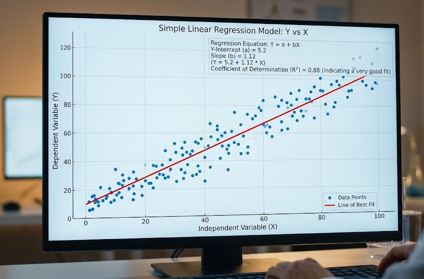
- Linear relationship: If the relationship between predictor and outcome appears linear on a scatter plot, standard linear regression is appropriate.
- Non-linear relationship: If the relationship curves, consider polynomial regression, spline models, or logarithmic/exponential regression. Plotting your data before modelling helps identify this.
3. Number of Predictors
- One predictor: Simple linear or logistic regression
- Multiple predictors: Multiple regression (also called multivariable regression); this is the norm in most biomedical studies, where controlling for confounders is essential
4. Checking Assumptions
Each regression type rests on assumptions. If these are violated, your estimates may be biased or inefficient.
| Assumption | What it means | How to test it |
| Linearity | The relationship between predictors and outcome is linear | Scatter plots; residual vs. fitted value plots |
| Homoscedasticity | Variance of residuals is constant across the range of fitted values | Residual vs. fitted value plot; Breusch-Pagan test |
| Independence of residuals | Observations are not clustered or correlated | Consider data structure; use mixed-effects models if patients are nested within sites |
| Normality of residuals | Residuals (not raw data) are approximately normally distributed | Q-Q plots; Shapiro-Wilk test |
| No perfect multicollinearity | Predictors are not perfectly correlated with each other | Variance inflation factor (VIF); values above 5–10 indicate a problem |
Note: A common misconception is that the outcome variable must be normally distributed. In linear regression, it is the residuals that should be approximately normal, not the raw data.
5. Handling Outliers
Outliers can disproportionately influence regression estimates, particularly in small biomedical datasets.
- Identify outliers using Cook’s distance, leverage plots, and standardised residual plots.
- If outliers are genuine data points (not errors), consider robust regression or weighted least squares rather than removing them.
- Document your approach to outlier handling transparently in your Methods section.
6. Multicollinearity Among Predictors
When two or more independent variables are strongly correlated (e.g., BMI and waist circumference), it becomes difficult to estimate their individual effects reliably.
- Calculate the variance inflation factor (VIF) for each predictor.
- If multicollinearity is severe, consider:
- Removing one of the correlated predictors on theoretical grounds
- Using ridge regression, which applies a penalty to shrink coefficients and stabilise estimates
- Using principal component regression to reduce dimensionality
7. Sample Size
Regression models require sufficient sample size to produce reliable estimates.
- For linear regression, a common rule of thumb is at least 10–20 observations per predictor variable.
- For logistic regression, the guideline is at least 10 events per predictor variable (EPV).
- With small samples, consider regularisation techniques such as ridge regression or LASSO regression, which reduce the risk of overfitting by penalising model complexity.
8. Data Distribution
- If your outcome variable is skewed, consider a data transformation (e.g., log transformation for right-skewed biological measures) before applying linear regression.
- Alternatively, use quantile regression, which models the median or other quantiles of the outcome rather than the mean, and is more robust to non-normal distributions and outliers.
- If standard assumptions cannot be met, robust regression methods provide more dependable estimates.
Understanding Regression Coefficients
Once your model is fitted, interpreting the output correctly is critical. Here is what the key elements mean in practice.
Linear Regression Output
In a linear regression model predicting systolic blood pressure (SBP):
SBP = 90 + 2.5(Age) + 4.1(BMI) + error
- The coefficient for Age (2.5) means: for every one-year increase in age, SBP increases by 2.5 mmHg, holding BMI constant.
- The coefficient for BMI (4.1) means: for every one-unit increase in BMI, SBP increases by 4.1 mmHg, holding age constant.
- The intercept (90) is the predicted SBP when both age and BMI equal zero (often not clinically meaningful, but required mathematically).
Logistic Regression Output
Logistic regression produces log-odds, which are typically converted to odds ratios (ORs) for clinical interpretation.
- An OR of 1.0 means no association between the predictor and the outcome.
- An OR greater than 1.0 means the odds of the outcome increase with that predictor.
- An OR less than 1.0 means the odds of the outcome decrease with that predictor.
Always report ORs alongside 95% confidence intervals. A confidence interval that includes 1.0 indicates the association is not statistically significant.
Statistical vs. Clinical Significance
A statistically significant result (p < 0.05) does not automatically mean a clinically meaningful one. In a large dataset, even a 0.2 mmHg increase in blood pressure per year may reach significance while being clinically irrelevant. Always interpret coefficients in the context of the clinical question.
Key Assumptions in Regression and How to Test Them
The validity of any regression model depends on its underlying assumptions being reasonably satisfied. Here is a practical checklist for the most common scenario (linear regression), with notes on other model types.
For linear regression
- Linearity: Plot each predictor against the outcome. Non-linear patterns suggest the need for transformation or polynomial terms.
- Homoscedasticity: In the residual vs. fitted plot, residuals should be scattered randomly around zero, with no funnel-shaped spread.
- Normality of residuals: Inspect a Q-Q plot. Minor departures from normality are usually acceptable in larger samples due to the central limit theorem.
- Independence: If your data include repeated measures, paired samples, or patients clustered within centres, standard regression will underestimate standard errors. Use mixed-effects models or GEE (generalised estimating equations) instead.
For logistic regression
- Check for linearity in the log-odds using the Box-Tidwell test or by inspecting fractional polynomial plots.
- Assess overall model fit using the Hosmer-Lemeshow test and examine the area under the ROC curve (AUC/c-statistic) as a measure of discrimination.
Common Mistakes in Regression Analysis
Researchers frequently encounter the following pitfalls:
- Overfitting: Including too many predictors relative to sample size produces a model that performs well on your dataset but generalises poorly. Use regularisation or limit predictors to those with a clear theoretical basis.
- Failing to validate assumptions: Running a regression without checking residual plots is one of the most common methodological errors flagged by peer reviewers.
- Ignoring multicollinearity: Including highly correlated predictors without checking VIF inflates standard errors and makes coefficients unreliable.
- Extrapolating beyond the data: Regression models should not be used to predict outcomes outside the range of the observed data used to build the model.
- Confusing association with causation: A statistically significant regression coefficient indicates association, not causation, unless the study is a properly randomised experiment.
- Not accounting for confounders: In observational biomedical studies, unadjusted (crude) regression estimates are frequently misleading. Always consider potential confounders and adjust accordingly.
See also: 6 best practices in regression analysis for biomedical researchers
How to Report Regression Results in a Research Paper
Transparent and complete reporting is increasingly scrutinised by journals and peer reviewers. The following guidance aligns with widely used reporting standards including STROBE (for observational studies) and CONSORT (for trials).
See also: How to report correlation and regression analyses in a research paper.
In the Methods Section, Report:
- The type of regression model used and the rationale for selecting it
- How the dependent variable and key predictors were defined and measured
- How assumptions were checked and what action was taken if they were violated
- How missing data were handled (complete-case analysis, multiple imputation, etc.)
- Whether a sample size or events-per-variable calculation was performed
- The statistical software and version used (e.g., R version 4.3.1, Stata 18)
In the Results Section, Report:
- Coefficients (or ORs/HRs for logistic/Cox models) with 95% confidence intervals for each predictor
- P-values, interpreted in conjunction with confidence intervals rather than in isolation
- The overall model fit statistic appropriate to your model type (R² for linear regression; AUC/c-statistic and Hosmer-Lemeshow for logistic regression; Harrell’s C-statistic for Cox regression)
- Both unadjusted and adjusted estimates where relevant, so readers can assess the impact of confounding
Example Table Format for Logistic Regression Results
| Predictor | Unadjusted OR (95% CI) | p-value | Adjusted OR (95% CI) | p-value |
| Age (per year) | 1.04 (1.02–1.07) | 0.001 | 1.03 (1.01–1.06) | 0.008 |
| BMI (per unit) | 1.12 (1.06–1.19) | <0.001 | 1.09 (1.02–1.16) | 0.010 |
| Current smoker | 2.31 (1.54–3.46) | <0.001 | 1.98 (1.29–3.03) | 0.002 |
| Female sex | 0.74 (0.51–1.08) | 0.12 | 0.79 (0.54–1.16) | 0.23 |
Note: Always specify in the table footnote which variables were included in the adjusted model.
Quick Reference: Choosing Your Regression Method
| Research scenario | Recommended regression type |
| Predicting a continuous outcome (e.g., HbA1c) from one or more predictors | Multiple linear regression |
| Predicting a binary outcome (e.g., disease recurrence: yes/no) | Logistic regression |
| Estimating time to an event (e.g., death, relapse) | Cox proportional hazards regression |
| Dependent variable is a count (e.g., number of relapses) | Poisson or negative binomial regression |
| Relationship is clearly non-linear | Polynomial regression or spline models |
| High multicollinearity among predictors | Ridge regression |
| Small sample or many predictors, risk of overfitting | LASSO or ridge regression |
| Outcome distribution is skewed or non-normal | Quantile regression or data transformation |
| Data with outliers that cannot be removed | Robust regression |
| Repeated measures or clustered data | Mixed-effects models or GEE |
Summary
Choosing the right regression method is not simply a technical decision: it is a scientific one. It requires you to think carefully about your research question, the nature of your outcome variable, your sample size, and the assumptions your data can reasonably support.
The key steps are:
- Define the type of your dependent variable first: this narrows your options immediately.
- Examine your data before modelling: plots reveal non-linearity, outliers, and distributional issues that should inform your method choice.
- Check assumptions after fitting: even the right model can produce invalid results if its assumptions are violated.
- Interpret results carefully: distinguish statistical from clinical significance, and report both adjusted and unadjusted estimates.
- Report transparently: include sufficient methodological detail for readers and reviewers to evaluate and replicate your analysis.
Regression analysis is iterative: the right model often emerges after testing, refining, and validating. Consulting a biostatistician early in the study design phase, not just at the analysis stage, can save considerable time and strengthen your manuscript considerably.
Unsure which regression method best fits your data and research question? Editage’s Statistical Analysis and Review Services connect you with expert biostatisticians who can guide your analysis from design through to publication.
This article was originally published on February 18, 2024, and updated on May 27, 2026.