Descriptive Statistics: A Comprehensive Guide for Biomedical Research
Key Takeaways
- Descriptive statistics summarize data without making inferences; they are distinct from but complementary to inferential statistics.
- The three main types of descriptive statistics are measures of central tendency, measures of variability, and frequency distributions.
- Choose mean ± SD for normally distributed data; median (IQR) for skewed or ordinal data; frequency (%) for categorical data.
- Graphical tools (histograms, box plots, scatter plots) are indispensable for understanding and communicating data distributions.
- SD measures spread of individual values; SEM measures precision of the mean estimate. Never confuse them.
- Proper reporting of descriptive statistics, including sample size, units, missing data, and distribution assessment, is a cornerstone of research integrity.
Contents
- What Are Descriptive Statistics?
- Types of Data in Biomedical Research
- Frequency Distribution
- Measures of Central Tendency
- Measures of Variability (Dispersion)
- Shape of Distribution: Skewness and Kurtosis
- Graphical Representation of Descriptive Data
- Worked Biomedical Example: Summarizing a Clinical Dataset
- Confidence Intervals and Their Relationship to Descriptive Statistics
- Percentiles and Quartiles in Biomedical Research
- Reporting Descriptive Statistics in Biomedical Research
- Applications of Descriptive Statistics Across Biomedical Disciplines
- Software Tools for Descriptive Statistics in Biomedical Research
- Frequently Asked Questions
- Conclusion
Descriptive statistics form the essential foundation of biomedical research. These summary measures (the means, medians, standard deviations, and frequency distributions) tell the story of a dataset in a concise, interpretable form.
In clinical studies, epidemiological surveys, laboratory investigations, and public health research, descriptive statistics help clinicians and scientists communicate their findings clearly. Whether you are analyzing blood pressure readings from a hypertension trial, survival times in an oncology study, or HbA1c trends in a diabetes management program, understanding descriptive statistics is the critical first step.
This comprehensive guide covers every major aspect of descriptive statistics with biomedical examples, comparison of measures, step-by-step calculation guidance, and best practices for reporting in peer-reviewed research.
What Are Descriptive Statistics?
Descriptive statistics are numerical and graphical tools that summarize and describe the main features of a dataset. They do not go beyond the data collected; instead, they present quantitative characteristics in a manageable, interpretable form.
Why Descriptive Statistics Matter in Biomedical Research
In biomedical contexts, raw datasets are rarely interpretable at face value. A dataset of 5,000 patient blood glucose values is meaningless without summary. Descriptive statistics transform complexity into clarity. They are important because they:
- Allow researchers to understand the distribution and spread of clinical measurements
- Help identify data quality issues, outliers, and entry errors before analysis
- Provide a clear characterization of the study population for journal reporting
- Serve as the basis for choosing appropriate inferential statistical tests
- Enable comparison of baseline characteristics between groups in randomized controlled trials
- Communicate findings to clinicians and policymakers without overwhelming technical detail
Descriptive vs. Inferential Statistics
Descriptive and inferential statistics serve fundamentally different purposes. Understanding the distinction is essential for proper study design and analysis.
| Feature | Descriptive Statistics | Inferential Statistics |
| Purpose | Summarize and describe data | Draw conclusions beyond the data |
| Scope | Describes the observed sample or population | Generalizes findings to a broader population |
| Hypothesis | No hypothesis testing involved | Tests hypotheses; computes p-values |
| Output | Mean, median, SD, frequency tables, charts | t-tests, ANOVA, regression, confidence intervals |
| Biomedical Example | Mean HbA1c = 7.4% in a diabetic cohort | Is HbA1c significantly lower after treatment? (p < 0.05) |
| Complexity | Simpler; first step in analysis | More complex; requires assumptions about distributions |
Key insight: Descriptive statistics describe what is; inferential statistics help you determine what might be true for the broader population. Both are necessary in a complete biomedical analysis. For example, a clinical trial report would use descriptive statistics to characterize the study population (Table 1 in most papers) and inferential statistics to assess treatment effects (p-values and confidence intervals in Table 2 onwards).
Types of Data in Biomedical Research
Before applying descriptive statistics, it is essential to understand the type of data being analyzed. Different data types require different descriptive measures. Misidentifying data type is one of the most common errors in biomedical statistical reporting.
| Data Type | Scale | Properties | Biomedical Example |
| Nominal | Categorical | No order; named categories only | Blood group (A, B, AB, O); disease presence (yes/no) |
| Ordinal | Categorical | Ordered categories; unequal intervals | Pain scale (mild, moderate, severe); cancer staging (I–IV) |
| Interval | Numerical | Equal intervals; no true zero | Body temperature in °C or °F; calendar year of diagnosis |
| Ratio | Numerical | Equal intervals; true zero exists | Blood glucose (mg/dL); height (cm); white blood cell count |
Continuous vs. Discrete Variables
- Continuous variables: Can take any value within a range. Examples include weight (kg), serum albumin (g/dL), and ejection fraction (%). These are described with mean, SD, and range.
- Discrete variables: Can only take whole-number values. Examples include number of hospital admissions, parity, or lesion count. These may be described with mean or median, plus range.
Univariate, Bivariate, and Multivariate Analysis
- Univariate analysis: Examines one variable at a time. Example: describing the distribution of serum creatinine in a nephrology cohort.
- Bivariate analysis: Examines the relationship between two variables. Example: comparing BMI between diabetic and non-diabetic patients.
- Multivariate analysis: Examines three or more variables simultaneously. Example: characterizing patients by age, gender, diagnosis, and comorbidities in a baseline table.
Frequency Distribution
A frequency distribution is a summary of how often each value or range of values occurs in a dataset. It is typically the first step in understanding the shape and structure of a dataset before applying any other descriptive or inferential methods.
Components of a Frequency Distribution
- Absolute frequency: The raw count of occurrences. Example: 45 patients had a BMI between 25 and 30 kg/m².
- Relative frequency: Proportion of cases; expressed as a percentage. Example: 22.5% of the study population had a BMI between 25 and 30.
- Cumulative frequency: Running total of proportions up to a given value. Example: 68% of patients had an HbA1c below 8%.
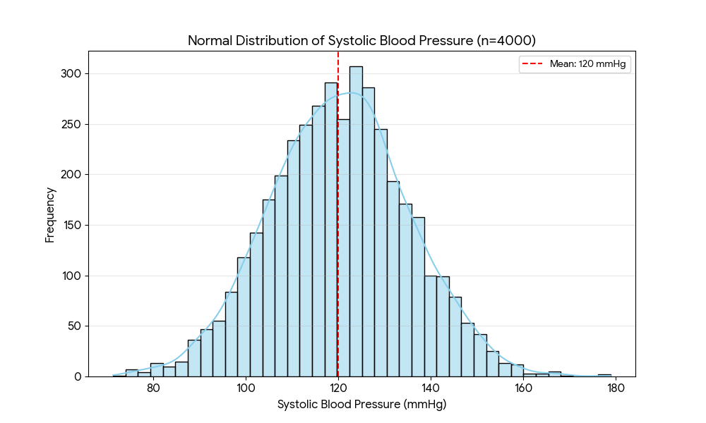
The Normal Distribution
In biomedical research, the normal (Gaussian) distribution is one of the most important concepts. Many biological measurements approximate normality, including:
- Height and weight in healthy adult populations
- Serum electrolyte levels (e.g., sodium, potassium) in stable outpatients
- Systolic blood pressure in large community-based surveys
When data follow a normal distribution:
- 68% of values fall within ±1 SD of the mean
- 95% of values fall within ±2 SD of the mean
- 99.7% of values fall within ±3 SD of the mean
Clinical relevance:
Reference ranges in laboratory medicine (e.g., hemoglobin, creatinine, platelet counts) are typically defined as the mean ± 2 SD of a healthy reference population, covering approximately 95% of normal values.
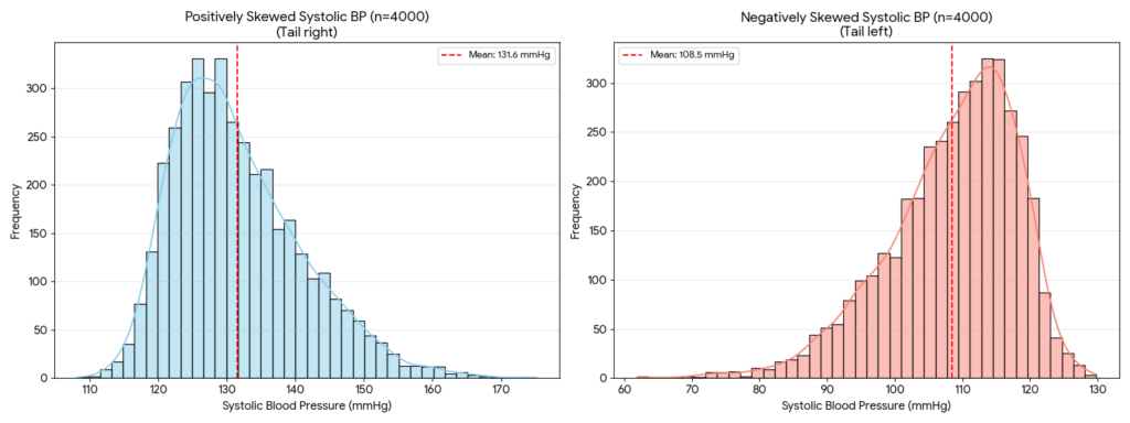
Skewed Distributions in Biomedical Data
Not all biomedical data are normally distributed. Many measurements are inherently skewed:
- Positively skewed (right-skewed): A few high values pull the tail to the right. Examples include hospital length of stay, serum CRP levels, and tumor marker concentrations. The mean > median in positively skewed data.
- Negatively skewed (left-skewed): A few low values pull the tail to the left. Examples include age at death in elderly cohorts and cognitive test scores in a high-performing group. The mean < median in negatively skewed data.
Practical implication:
When data are skewed, the median is a more representative measure of central tendency than the mean, and the IQR is a more appropriate measure of spread than the SD.
Measures of Central Tendency
Measures of central tendency estimate the center or typical value of a dataset. The three primary measures, mean, median, and mode, each have distinct properties and optimal use cases in biomedical research. The geometric mean is also used for specific types of biological data.
| Measure | Definition | Best Used When | Biomedical Example |
| Mean | Sum of all values divided by n | Data is normally distributed, no extreme outliers | Mean systolic BP = 128 mmHg in a hypertension trial |
| Median | Middle value in an ordered dataset | Skewed data or presence of outliers | Median survival time = 18 months in a cancer cohort |
| Mode | Most frequently occurring value | Categorical or nominal data | Most common blood type in donors = O positive |
| Geometric Mean | nth root of the product of n values | Log-normally distributed data (e.g., antibody titers) | Geometric mean titer = 320 IU/mL for vaccine response |
Calculating the Mean
The arithmetic mean is calculated by summing all observations and dividing by the total count.
Formula:
μ = (Σx) / n
Example: In a study of 6 patients, fasting blood glucose values (mg/dL) were: 92, 105, 118, 88, 130, 97.
| Step | Calculation |
| 1. Sum all values | 92 + 105 + 118 + 88 + 130 + 97 = 630 |
| 2. Count observations (n) | n = 6 |
| 3. Divide sum by n | Mean = 630 / 6 = 105 mg/dL |
Calculating the Median
The median is identified after ordering all data points from smallest to largest. If n is odd, the median is the middle value. If n is even, it is the average of the two middle values.
Using the same glucose values: Ordered: 88, 92, 97, 105, 118, 130
- Two middle values: 97 and 105
- Median: (97 + 105) / 2 = 101 mg/dL
Note: The mean (105 mg/dL) and median (101 mg/dL) differ slightly, suggesting a mild positive skew driven by the high value of 130 mg/dL.
When to Use Mean vs. Median
The choice between mean and median is one of the most important decisions in descriptive reporting:
- Use the mean when data are normally distributed (e.g., serum sodium in stable patients, height in adult populations).
- Use the median when data are skewed, when outliers are present, or when the variable has a natural floor or ceiling (e.g., survival time, length of stay, pain scores).
- For categorical or ordinal data, use the mode or frequency distribution rather than mean or median.
The Geometric Mean in Biomedical Research
The geometric mean is the appropriate measure of central tendency for data that is log-normally distributed. This is common in:
- Serological antibody titers (e.g., vaccine immunogenicity studies)
- Viral load measurements (e.g., HIV RNA copies/mL)
- Cytokine concentrations (e.g., IL-6, TNF-α in inflammatory studies)
- Pharmacokinetic parameters such as area under the curve (AUC)
Formula:
Geometric Mean = (x₁ × x₂ × … × xₙ)¹ⁿ; equivalently, the antilog of the mean of the log-transformed values.
Measures of Variability (Dispersion)
Knowing only the average of a dataset is insufficient. Two clinical populations can have identical means yet very different distributions. Measures of variability describe how spread out or dispersed the data are, providing crucial context for interpreting central tendency values.
| Measure | Definition | Formula | Biomedical Example |
| Range | Difference between max and min values | Max – Min | BMI range in study: 17.2 to 42.6 kg/m² |
| Variance (s²) | Average of squared deviations from the mean | Σ(x−μ)² / (n−1) | Variance in fasting glucose values across 200 subjects |
| Standard Deviation (SD) | Square root of variance; average spread around mean | √[Σ(x−μ)² / (n−1)] | Mean cholesterol = 195 mg/dL, SD = 28 mg/dL |
| IQR | Range of the middle 50% of values (Q3 – Q1) | Q3 – Q1 | IQR of hospital stay duration = 3–7 days |
| CV (%) | SD as a percentage of the mean | (SD / Mean) × 100 | CV of lab assay = 4.2%; assay is precise |
| SEM | Precision of the sample mean estimate | SD / √n | SEM of treatment group mean = ±1.3 mg/dL |
Standard Deviation: Step-by-Step Calculation
Standard deviation (SD) is the most widely used measure of variability in biomedical research. Using the 6 glucose values: 92, 105, 118, 88, 130, 97 (mean = 105 mg/dL):
| Value (x) | x − μ | (x − μ)² | Running note |
| 92 | 92−105 = −13 | 169 | Below average |
| 105 | 0 | 0 | At the mean |
| 118 | +13 | 169 | Above average |
| 88 | −17 | 289 | Lowest value; furthest from mean |
| 130 | +25 | 625 | Highest value; furthest from mean |
| 97 | −8 | 64 | Below average |
| Sum | Σ = 0 | Σ = 1316 | Sum of deviations always = 0 |
- Variance (s²) = 1316 / (6 − 1) = 1316 / 5 = 263.2 (mg/dL)²
- SD (s) = √263.2 = 16.2 mg/dL
- Interpretation: On average, individual glucose values deviate from the mean by approximately 16.2 mg/dL.
SD vs. SEM: A Critical Distinction
One of the most frequently misused statistics in biomedical literature is the confusion between standard deviation (SD) and standard error of the mean (SEM). These measure fundamentally different things:
- SD measures the spread of individual observations around the sample mean. It describes the variability within the sample or population. Use SD when describing the distribution of a clinical measurement in your sample.
- SEM measures the precision of the sample mean as an estimate of the true population mean. SEM = SD / √n. It shrinks as sample size increases. Use SEM when reporting confidence around a mean estimate.
Caution:
Using SEM instead of SD makes variability appear smaller and data more precise than it actually is. Most biomedical journals require SD for descriptive reporting in Table 1.
The Coefficient of Variation (CV)
The CV is particularly useful in biomedical laboratory science for assessing assay precision and comparing variability across measurements with different units.
Formula: CV (%) = (SD / Mean) × 100
Example applications:
- A laboratory assay with CV < 5% is considered highly precise and reproducible.
- Comparing variability in blood glucose (mean = 120 mg/dL, SD = 15) vs. body weight (mean = 75 kg, SD = 10 kg): CV for glucose = 12.5%; CV for weight = 13.3% — comparable relative variability despite different units.
The Interquartile Range (IQR)
The IQR is the range containing the middle 50% of data values (from the 25th percentile, Q1, to the 75th percentile, Q3). It is resistant to outliers, making it preferable over the range for skewed biomedical data.
Example: In a study of pediatric length of hospital stay:
- Q1 = 3 days; Q3 = 9 days; IQR = 6 days
- This means 50% of children stayed between 3 and 9 days.
- One extreme outlier (stay of 120 days) does not affect the IQR, though it greatly inflates the range.
Shape of Distribution: Skewness and Kurtosis
Beyond central tendency and spread, the shape of a distribution provides important information about the nature of biomedical data and guides the selection of appropriate statistical tests.
| Parameter | Value Range | Interpretation | Biomedical Example |
| Skewness = 0 | Exactly 0 | Perfectly symmetrical (normal distribution) | Height distribution in a homogeneous cohort |
| Positive Skew | > 0 | Right tail is longer; most values cluster on the left | Serum creatinine in healthy individuals |
| Negative Skew | < 0 | Left tail is longer; most values cluster on the right | Age at death in a geriatric cohort |
| Leptokurtic | Kurtosis > 3 | Heavy tails; more extreme outliers than normal | Drug concentration spikes in pharmacokinetic data |
| Platykurtic | Kurtosis < 3 | Light tails; fewer extreme values than normal | Uniform distribution of lab testing errors |
Clinical Significance of Skewness
Understanding skewness helps clinicians and researchers avoid statistical misinterpretation:
- Right-skewed data: Common for biological concentrations (CRP, ferritin, troponin), healthcare utilization metrics (ED visits, readmissions), and time-to-event data (survival, time to recovery). Always report median and IQR.
- Left-skewed data: Less common; seen in age-at-death distributions in elderly populations and high-pass test scores. Use median and IQR.
- Symmetric data: Height, blood pressure in large samples, and many laboratory values in healthy cohorts. Mean and SD are appropriate.
Assessing Normality
Before applying parametric statistical tests, normality should be formally assessed. Methods include:
- Visual inspection: histogram, Q-Q plot (quantile-quantile plot), box plot
- Statistical tests: Shapiro-Wilk test (preferred for small samples, n < 50); Kolmogorov-Smirnov test (for larger samples)
- Skewness and kurtosis values: If skewness and kurtosis z-scores fall within ±2, data may be considered approximately normal
Graphical Representation of Descriptive Data
Data visualization is an indispensable component of descriptive statistics. Graphs translate numerical summaries into intuitive visual formats, making patterns, outliers, and distributions immediately apparent.
| Graph Type | Best For | Biomedical Example |
| Histogram | Continuous variable frequency distribution | Distribution of diastolic BP values across 500 patients |
| Box Plot | Spread, median, and outliers | Comparing LDL levels across three treatment arms |
| Bar Chart | Comparing categorical groups | Frequency of adverse events by drug dose level |
| Pie Chart | Proportions of a whole | Proportion of patients by cancer stage at diagnosis |
| Scatter Plot | Relationship between two continuous variables | Correlation between BMI and fasting insulin levels |
| Line Graph | Trends over time | Weekly mean hemoglobin during a 12-week iron therapy trial |
| Frequency Table | Exact counts and proportions for any variable | Distribution of comorbidities in a diabetic population |
Choosing the Right Graph
Selecting an inappropriate graph type is a common error in biomedical publications. The following guidance applies:
- One continuous variable: Use a histogram to display the distribution, or a box plot for compact summaries across groups.
- One categorical variable: Use a bar chart (for counts) or pie chart (for proportions).
- Two continuous variables: Use a scatter plot to visualize the relationship.
- One variable over time: Use a line graph to show trends.
- Comparing groups: Use side-by-side box plots for continuous outcomes (e.g., comparing serum creatinine between CKD stages).
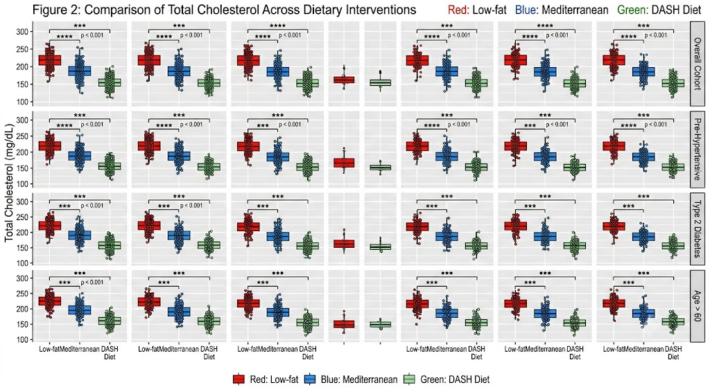
Box Plots in Biomedical Research
Box plots (box-and-whisker plots) are particularly valuable in clinical research because they simultaneously display:
- The median (central line within the box)
- The IQR (the box itself, spanning Q1 to Q3)
- The range (whiskers extending to 1.5× IQR beyond Q1 and Q3)
- Outliers (individual points beyond the whiskers)
Example: A box plot comparing total cholesterol across three dietary intervention groups (low-fat, Mediterranean, and DASH diet) immediately reveals differences in median, spread, and outlier presence across groups. This is information that a simple table of means cannot convey.
Worked Biomedical Example: Summarizing a Clinical Dataset
The following example demonstrates how descriptive statistics are applied in a real-world clinical research scenario. This is the kind of summary table (Table 1) that appears in virtually every original research article.
Study Scenario
A cross-sectional study enrolls 500 adults with type 2 diabetes from a tertiary hospital. Researchers collected demographic and clinical data including age, systolic blood pressure (SBP), glycated hemoglobin (HbA1c), and BMI.
| Variable | Mean (SD) | Median (IQR) | Range | Distribution |
| Age (years) | 52.3 (11.6) | 51.0 (43–61) | 28–81 | Approximately normal |
| Systolic BP (mmHg) | 138.4 (18.2) | 136 (124–152) | 90–200 | Slight positive skew |
| HbA1c (%) | 7.8 (1.4) | 7.6 (6.9–8.5) | 5.2–14.3 | Right-skewed |
| BMI (kg/m²) | 28.9 (5.7) | 28.1 (25.0–32.3) | 17.2–42.6 | Slightly right-skewed |
| Gender (Female) | N/A | N/A | N/A | 54% female (n=270) |
Interpreting the Results
- Age is approximately normally distributed (mean ≈ median), so reporting mean ± SD is appropriate.
- Systolic BP has a slight positive skew (mean slightly > expected median), but both mean±SD and median(IQR) are reported for completeness.
- HbA1c is right-skewed (mean > median), which is common in diabetic cohorts with some poorly controlled patients. The median and IQR are the primary descriptors.
- BMI is slightly right-skewed, again common in clinical populations. Median(IQR) is preferred.
- Gender is a nominal categorical variable. Descriptive reporting uses count and percentage; mean/SD and median/IQR are not applicable.
Confidence Intervals and Their Relationship to Descriptive Statistics
While confidence intervals (CIs) are technically inferential tools, they are routinely reported alongside descriptive statistics in biomedical literature and play an important role in interpreting sample-level summaries.
What Is a Confidence Interval?
Definition: A 95% confidence interval means that if the same study were repeated 100 times using random samples from the same population, approximately 95 of those intervals would contain the true population mean.
Example: In a hypertension trial, the mean SBP reduction after 12 weeks of treatment = 14.2 mmHg, 95% CI: 11.8 to 16.6 mmHg.
- The CI tells us that the true mean reduction is likely between 11.8 and 16.6 mmHg.
- A narrower CI indicates greater precision (larger sample or lower variability).
- A CI that does not cross zero indicates a statistically significant result at α = 0.05.
CI Formula for a Mean
95% CI = Mean ± (1.96 × SEM), where SEM = SD / √n
Example: Mean HbA1c = 7.8%, SD = 1.4%, n = 500
- SEM = 1.4 / √500 = 1.4 / 22.4 = 0.063
- 95% CI = 7.8 ± (1.96 × 0.063) = 7.8 ± 0.12 = [7.68%, 7.92%]
Percentiles and Quartiles in Biomedical Research
Percentiles divide an ordered dataset into 100 equal parts. They are widely used in clinical medicine for defining normal ranges, growth standards, and population benchmarks.
Key Percentile Definitions
- 25th percentile (Q1): 25% of values fall below this point. Used as the lower boundary of the IQR.
- 50th percentile (Q2 / Median): 50% of values fall below this point. The middle of the distribution.
- 75th percentile (Q3): 75% of values fall below this point. Used as the upper boundary of the IQR.
- 90th, 95th, 97th percentiles: Used in pediatric growth charts (weight, height, head circumference) to define normal growth.
Clinical Applications of Percentiles
- Pediatric growth monitoring: A child’s weight falling below the 3rd percentile for age may indicate failure to thrive and warrants investigation.
- Reference ranges: Many clinical chemistry laboratories define normal values as the 2.5th to 97.5th percentile of a healthy reference population (central 95%).
- Blood pressure classification: Hypertension in pediatric patients is defined as SBP or DBP ≥ 95th percentile for age, sex, and height.
- Nutritional assessment: Mid-upper arm circumference (MUAC) below the 5th percentile is used to screen for acute malnutrition in field settings.
Reporting Descriptive Statistics in Biomedical Research
Accurate and transparent reporting of descriptive statistics is a core requirement of good scientific practice. Many journals and reporting guidelines (e.g., CONSORT, STROBE, TRIPOD) specify how descriptive data should be presented.
General Reporting Principles
- Always report n (sample size) clearly, including the number of missing observations per variable.
- Report mean ± SD for normally distributed continuous variables (e.g., height, weight, blood pressure in large community samples).
- Report median (IQR) for skewed or ordinal variables (e.g., length of stay, pain scores, tumor markers).
- Report frequency and percentage [n (%)] for categorical variables (e.g., gender, disease stage, smoking status).
- Always specify measurement units (e.g., mg/dL, mmHg, kg/m²) for all clinical variables.
- Distinguish clearly between SD and SEM in figure legends and table footnotes.
- For time-to-event data (survival analysis), report the median survival time with 95% CI rather than the mean.
Reporting Checklist for Biomedical Descriptive Statistics
| Reporting Element | Guidance / Example |
| Sample size and completeness | State total N and missing data per variable |
| Appropriate central tendency | Use mean ± SD for normal data; median (IQR) for skewed |
| Data distribution assessed | Report skewness, kurtosis, or normality test results |
| SD vs. SEM clearly distinguished | SD describes spread of data; SEM describes precision of mean |
| Graphical representation included | Histograms, box plots, or scatter plots as appropriate |
| Outliers identified and addressed | Report outliers; explain inclusion/exclusion decisions |
| Confidence intervals reported | Report 95% CI alongside point estimates where relevant |
| Units and scale provided | Always specify measurement units (e.g., mg/dL, mmHg, kg) |
Common Errors to Avoid
Several systematic errors in descriptive statistics reporting can mislead readers:
- Using SEM instead of SD to make data appear more precise than it is.
- Reporting mean ± SD for heavily skewed data such as CRP, ferritin, or hospital admissions.
- Misidentifying ordinal data (pain scales, Likert scales, cancer staging) as continuous and computing a mean.
- Failing to report the number of missing values, leading to inflated or biased summary statistics.
- Overclaiming based on descriptive data alone without acknowledging the need for inferential testing.
- Using a pie chart for more than 5 categories, making visual comparison nearly impossible.
If you’re looking for an expert statistical analysis service to support you in choosing and analyzing descriptive statistics, book a conversation with our expert consultant today.
Applications of Descriptive Statistics Across Biomedical Disciplines
Descriptive statistics are universally applied across every domain of biomedical research. The following summaries highlight domain-specific uses:
Clinical Trials
Table 1 in every clinical trial is a purely descriptive table characterizing the study population at baseline. It typically includes:
- Demographic variables: age, sex, race/ethnicity
- Clinical measures: BMI, blood pressure, HbA1c, eGFR, LVEF
- Comorbidities: prevalence of hypertension, dyslipidemia, CKD, prior MI
- Medications: current drug use by class
The purpose is to allow readers to assess balance between treatment arms and to evaluate the generalizability of findings to their own patient population.
Epidemiology and Public Health
In epidemiological studies, descriptive statistics are used to:
- Calculate incidence rates (new cases per 1,000 person-years)
- Estimate prevalence (proportion of a population with a condition at a given point in time)
- Characterize demographic and risk factor distributions in population-based surveys
- Monitor trends over time (e.g., rising obesity prevalence, declining smoking rates)
Example: The National Family Health Survey (NFHS-5) in India reported descriptive statistics showing that 24% of women aged 15–49 years were overweight or obese (BMI ≥ 25 kg/m²), up from 21% in NFHS-4. This is a purely descriptive finding with major public health significance.
Laboratory Medicine and Pathology
Descriptive statistics are fundamental to laboratory medicine for:
- Establishing and validating reference intervals for analytes (e.g., serum creatinine, hemoglobin, TSH)
- Monitoring assay precision and accuracy using CV, Levey-Jennings charts, and Westgard rules
- Describing histopathological findings (e.g., median Ki-67 index in breast cancer specimens)
- Analyzing quality control data for accreditation purposes
Pharmacology and Drug Development
- Describing pharmacokinetic parameters across dose groups: mean AUC, C_max, t_1/2
- Summarizing adverse event profiles: incidence, severity distribution, time to onset
- Characterizing dose-response relationships in Phase II trials
- Reporting geometric mean ratios in bioequivalence studies
Genomics and Biomarker Research
- Describing gene expression levels (often log-transformed due to skewness)
- Summarizing biomarker concentrations across patient subgroups
- Presenting allele frequency distributions in genome-wide association studies (GWAS)
- Characterizing sequencing read depth distributions in next-generation sequencing (NGS) datasets
Software Tools for Descriptive Statistics in Biomedical Research
Numerous software tools are available for computing and visualizing descriptive statistics. The choice of software often depends on the researcher’s background, data type, and institutional resources.
| Software | Key Features | Best For | Notes |
| SPSS | GUI-based, comprehensive output, tables and charts | Clinical researchers, non-programmers | Standard in health sciences; produces publication-ready tables |
| R | Free, open-source, powerful visualization (ggplot2) | Epidemiologists, biostatisticians | Packages: tableone, psych, Hmisc for descriptive tables |
| Python | Pandas, NumPy, SciPy, Matplotlib, Seaborn | Computational researchers, data scientists | Excellent for large datasets and automation |
| SAS | PROC MEANS, PROC FREQ, PROC UNIVARIATE | Pharmaceutical industry, regulatory submissions | Industry standard for FDA submissions; robust and validated |
| Stata | Summarize, tabulate, histogram commands | Epidemiology, health economics | Widely used in observational research and global health |
| Excel | Data Analysis ToolPak, pivot tables | Small datasets, quick summaries | Accessible but limited for complex analyses; error-prone |
Key Functions for Descriptive Statistics in R
For researchers using R, the following functions provide efficient descriptive analysis:
- summary(data): Provides min, Q1, median, mean, Q3, max for each variable
- describe() from the Hmisc package: Comprehensive descriptive statistics with missing data counts
- CreateTableOne() from the tableone package: Automatically generates publication-ready Table 1 stratified by group
- ggplot2::geom_histogram() and geom_boxplot(): High-quality visualizations for distributions
Frequently Asked Questions
What is the difference between a parameter and a statistic?
A parameter describes a characteristic of an entire population (e.g., the true mean blood pressure of all adults in a country). A statistic describes a characteristic of a sample drawn from that population (e.g., the mean blood pressure of 500 adults enrolled in a study). Descriptive statistics summarize statistics (sample-level values); inferential statistics use those statistics to estimate parameters.
When should I use the geometric mean?
Use the geometric mean when your data spans several orders of magnitude or follows a log-normal distribution. This is common for immunological data (antibody titers), microbiological counts (colony-forming units), pharmacokinetic parameters (AUC, Cmax), and environmental exposure measurements. The geometric mean is always ≤ the arithmetic mean for positive values.
How many decimal places should I report?
As a general rule, report one more decimal place than the precision of the original measurement. For example:
- If weight is measured in whole kilograms, report the mean to one decimal place (e.g., 72.4 kg).
- If blood pressure is measured to the nearest 2 mmHg, report the mean to one decimal place.
- For percentages based on small samples, report to zero or one decimal place. Do not report 33.333% if n = 3.
Can descriptive statistics prove causation?
No. Descriptive statistics can reveal patterns, associations, and differences in data, but they cannot establish causality. Causal inference requires appropriate study design (e.g., randomized controlled trials, natural experiments) and inferential analysis. A descriptive finding that patients with higher BMI have higher HbA1c values does not prove that obesity causes diabetes; confounders, reverse causality, and selection bias must all be considered.
What is the difference between population variance and sample variance?
Population variance (σ²): Divides the sum of squared deviations by N (the total population size). Used only when you have complete population data.
Sample variance (s²): Divides by n−1 (Bessel’s correction). Used when working with a sample drawn from a larger population, which is nearly always the case in biomedical research. This correction makes the sample variance an unbiased estimator of the population variance.
This article was originally published on March 1, 2023, and updated on June 5, 2026.


Comment