Heteroskedasticity vs. Homoskedasticity: Definition and Examples
In this article, you’ll learn
- Why Should You Care About Variance?
- What Is Homoscedasticity?
- What Is Heteroscedasticity?
- A Side-by-Side Comparison: Homoskedasticity vs Heteroskedasticity
- Why Does Heteroskedasticity Matter in Biomedical Research?
- How to Detect Heteroscedasticity
- What to Do When You Find Heteroscedasticity
- A Quick Decision Framework
- Common Mistakes to Avoid Regarding Heteroskedasticity
- Key Takeaways
Why Should You Care About Variance?
Imagine you’re measuring blood glucose levels in 200 patients: half healthy controls, half with Type 2 diabetes. You run a regression analysis, feel confident in your results, and report them in your lab report. But your supervisor flags an issue: “Did you check the residuals?”
This is where homoscedasticity and heteroscedasticity come in. These concepts describe how the spread (variance) of your data behaves across different conditions or values. Getting this wrong can silently invalidate your statistical conclusions, even when your p-values look statistically significant.
What Is Homoscedasticity?
Homoscedasticity (from Greek: homos = same, skedasis = dispersion) means that the variance of your residuals (i.e., the differences between observed and predicted values) remains roughly constant across all levels of your predictor variable.
In plain English: the data points are spread out to a similar degree no matter where you look along your regression line.
Key characteristics of homoscedastic data:
- Residuals form a consistent, even “band” around the regression line
- No systematic fanning or narrowing of data points
- A core assumption of Ordinary Least Squares (OLS) regression, ANOVA, and many other parametric tests
- Produces reliable standard errors, valid p-values, and trustworthy confidence intervals
What Is Heteroscedasticity?
Heteroscedasticity (hetero = different) is the opposite: the variance of residuals changes at different levels of the predictor. The spread of your data is uneven: it might be tight in one region and wide in another.
Key characteristics of heteroscedastic data:
- Residuals fan out (or funnel in) as the predictor value increases
- Variance is not constant; it depends on the value of X
- Violates a fundamental assumption of many standard statistical tests
- Can lead to biased standard errors, inflated or deflated t-statistics, and misleading p-values
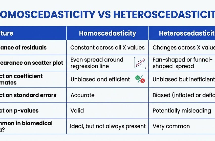
A Side-by-Side Comparison: Homoskedasticity vs Heteroskedasticity
| Feature | Homoscedasticity | Heteroscedasticity |
| Variance of residuals | Constant across all X values | Changes across X values |
| Appearance on scatter plot | Even spread around regression line | Fan-shaped or funnel-shaped spread |
| Effect on coefficient estimates | Unbiased and efficient | Unbiased but inefficient |
| Effect on standard errors | Accurate | Biased (inflated or deflated) |
| Effect on p-values | Valid | Potentially misleading |
| Common in biomedical data? | Ideal, but not always present | Very common |
Why Does Heteroskedasticity Matter in Biomedical Research?
Biomedical data is especially prone to heteroscedasticity. Here’s why:
- Biological variability scales with magnitude. A patient with a very high C-reactive protein (CRP) level will naturally show more variability in repeated measurements than a healthy individual with near-zero CRP.
- Measurement error scales with the instrument. Many lab assays have error that is proportional to the true value, which is a classic source of heteroscedasticity.
- Populations are heterogeneous. Age, body mass, comorbidities, and genetics all interact, making variance non-uniform across subgroups.
Real-World Biomedical Examples
- Pharmacokinetics: Drug plasma concentration often shows higher variance at higher doses, creating a characteristic fan shape when plotted against time or dose.
- Genomics (RNA-seq data): Highly expressed genes tend to have much greater absolute variability than lowly expressed genes. This is why specialized methods like DESeq2 and edgeR were developed rather than applying standard linear models.
- Blood pressure studies: Variance in systolic blood pressure readings tends to increase in hypertensive populations compared to normotensive controls.
- Body weight and metabolic markers: Heavier patients typically show more spread in fasting insulin, triglycerides, and HbA1c values.
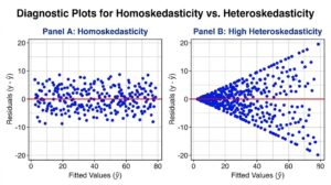
How to Detect Heteroscedasticity
Visual Inspection (Always Do This First)
The quickest diagnostic is a residual vs. fitted plot:
- Run your regression model
- Plot the residuals (Y-axis) against the fitted (predicted) values (X-axis)
- Look for patterns
What you’re looking for:
- ✅ Homoscedastic: Points randomly scattered in a horizontal band with no pattern
- ❌ Heteroscedastic: A cone or funnel shape; variance clearly increases or decreases
A scale-location plot (square root of standardized residuals vs. fitted values) is another useful visual tool and is standard output in R’s plot(model) function.
Formal Statistical Tests
When visual inspection is ambiguous, formal tests provide confirmation:
| Test | What It Does | Best Used When |
| Breusch-Pagan Test | Regresses squared residuals on predictors; detects linear heteroscedasticity | General-purpose; widely used |
| White’s Test | A more general version of Breusch-Pagan; detects non-linear patterns too | Complex models with interactions |
| Goldfeld-Quandt Test | Splits data in two and compares variances | Variance changes at a known breakpoint |
| Levene’s Test | Compares variance across groups | ANOVA settings; comparing group variances |
Interpreting the results:
- A significant p-value (typically < 0.05) in these tests indicates heteroscedasticity is present
- These tests can be overly sensitive in large samples so always combine with visual inspection
What to Do When You Find Heteroscedasticity
Finding heteroscedasticity is not a catastrophe. It’s just a signal to adapt your approach. Here are your main options:
Option 1: Transform Your Outcome Variable
This is often the first line of defense. Common transformations include:
- Log transformation: works well for right-skewed, multiplicative data (e.g., cytokine concentrations, enzyme activity levels)
- Square root transformation: useful for count data (e.g., cell counts, colony-forming units)
- Reciprocal (1/Y): appropriate for rate data where extreme values are problematic
Caveat: Transformations change the scale of your results, which can complicate interpretation. Always back-transform when reporting means.
Option 2: Use Weighted Least Squares (WLS)
Instead of treating all data points equally, WLS assigns lower weight to observations with higher variance. This corrects for heteroscedasticity while keeping data on the original scale.
- Weights are typically set as the inverse of the estimated variance
- Particularly useful in clinical studies where some measurements are less reliable than others
Option 3: Use Robust Standard Errors
Also called heteroscedasticity-consistent (HC) standard errors or “sandwich estimators,” this approach keeps your coefficient estimates the same but corrects the standard errors to be valid in the presence of heteroscedasticity.
- Available in most statistical software (e.g., vcovHC() in R, robust option in Stata)
- A practical choice when you want to stay on the original scale and don’t want to respecify your model
Option 4: Use a Generalized Linear Model (GLM)
For certain data types, a GLM with an appropriate distribution and link function naturally handles non-constant variance:
- Poisson or negative binomial regression for count data
- Gamma regression for continuous positive data with multiplicative variance
- Beta regression for proportions and fractions
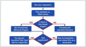
A Quick Decision Framework for Heteroskedasticity
Common Mistakes to Avoid Regarding Heteroskedasticity
- Ignoring it entirely. Heteroscedasticity does not bias your slope estimates, so the model may look fine but your inference (p-values, confidence intervals) will be wrong.
- Over-relying on tests alone. Formal tests have limited power in small samples and too much power in very large ones. Always pair them with visual diagnostics.
- Applying log transformation without checking. Log transforms help when variance scales with the mean, but can introduce problems if your data contains zeros or negative values.
- Forgetting to report it. In biomedical publications, documenting how you handled heteroscedasticity strengthens your methods section and reproducibility.
Key Takeaways
- Homoscedasticity = constant variance across predictor values. It’s an assumption, not a guarantee — always verify it.
- Heteroscedasticity = unequal variance. It’s extremely common in biomedical research and does not mean your data is “bad.”
- Detecting it requires both visual diagnostics (residual plots) and formal tests (Breusch-Pagan, Levene’s, etc.).
- Remedies include data transformations, weighted least squares, robust standard errors, and GLMs. The right choice depends on your data structure and research question.
- Reporting and addressing heteroscedasticity is a hallmark of rigorous, reproducible biomedical research.
This article was originally published on October 23, 2024, and updated on April 11, 2026.