Infographic: How to analyze count data in research


Contents
- What is count data?
- Related Statistical Concepts Glossary
- How to analyze count data?
- Comparison Table: Choosing the Right Test for Count Data
- Assumptions and Violations of Count Data Tests
- Step-by-Step How-To for Each Test
- Limitations of Each Test
- Reporting Results of Count Data Analysis in a Manuscript
- Real-World Examples of Count Data Analysis by Research Field
- Frequently Asked Questions
What is count data?
Count data refers to numerical values that represent the frequency or occurrence of discrete events. These events often involve the counting of specific entities, such as cells, disease cases, or genetic mutations. In the context of biomedical research, count data can be thought of as the number of times an event of interest occurs within a defined sample or population.
Count Data vs. Other Data Types
Understanding whether your data qualifies as count data is an important step before choosing a statistical test. Count data is often confused with other data types, which can lead to incorrect analysis choices.
What makes data “count data”?
- It consists of non-negative integers (0, 1, 2, 3, …)
- It represents the number of times a discrete event occurred
- There is a meaningful lower bound of zero, but no fixed upper bound in most cases
- Examples: number of hospital readmissions, number of mutations detected, number of adverse events
Count Data vs. Continuous Data
| Feature | Count Data | Continuous Data |
| Values | Non-negative integers only | Any real number within a range |
| Examples | Number of tumour cells, number of infections | Blood pressure, body weight, temperature |
| Distribution | Poisson or negative binomial | Normal (Gaussian) or other continuous distributions |
| Appropriate tests | Chi-square, Poisson regression, negative binomial regression | t-test, ANOVA, linear regression |
| Can it be negative? | No | Yes (depending on the variable) |
Count Data vs. Ordinal Data
| Feature | Count Data | Ordinal Data |
| Values | Actual numerical counts | Ranked categories (e.g., low, medium, high) |
| Examples | Number of relapses | Pain score on a 1-5 scale, disease severity rating |
| Mathematical operations | Addition and subtraction are meaningful | Ranking order is meaningful but differences between levels are not |
| Appropriate tests | Poisson or negative binomial regression | Ordinal logistic regression, Wilcoxon signed-rank test |
Count Data vs. Binary/Categorical Data
| Feature | Count Data | Binary/Categorical Data |
| Values | Non-negative integers | Fixed categories (yes/no, group A/B/C) |
| Examples | Number of seizures per month | Whether a patient has a disease (yes/no) |
| Appropriate tests | Poisson regression, negative binomial regression | Chi-square, Fisher’s exact test, logistic regression |
Common Mistakes in Classifying Data Types
- Treating count data as continuous and applying a t-test or linear regression, which can violate distributional assumptions and produce biased results
- Categorising count data into groups (e.g., low/high) unnecessarily, which loses information
- Confusing a Likert scale response (ordinal) with count data simply because both consist of integers
- Applying a chi-square test to data with very small sample sizes instead of Fisher’s exact test
Where is count data used in research?
Count data is extensively used in various areas of biomedical research. For example, in epidemiology, researchers may count the number of individuals with a particular disease in a population, while in genomics, scientists often count the occurrences of specific genetic variants or the expression levels of genes. In clinical research, counting adverse events or patient outcomes is common.
Related Statistical Concepts Glossary
Before we dive into analyzing count data, let’s define some of the key terms you’re going to find in this article.
| Term | Definition | Example |
| Count data | Non-negative integers representing how many times a discrete event occurred | Number of hospital visits, number of mutations, number of adverse events |
| Discrete distribution | A probability distribution describing outcomes that can only take specific, separate values (usually integers) | Poisson and negative binomial distributions, as opposed to the normal distribution |
| Poisson distribution | Models the number of events occurring in a fixed interval, assuming events occur independently at a constant average rate; the mean and variance are equal (both equal lambda) | Number of new infections per week in a stable epidemic |
| Negative binomial distribution | An extension of the Poisson distribution with an additional dispersion parameter that allows variance to exceed the mean | Used when count data is overdispersed, such as hospital readmissions in a high-risk population |
| Overdispersion | A condition where the variance of a count variable is greater than its mean, violating Poisson regression assumptions | A dataset of patient readmissions where a small number of patients account for a disproportionately high number of events |
| Zero-inflation | A condition where a dataset contains more zero counts than a standard Poisson or negative binomial model would predict | Species count surveys where most sites record no observations of a rare animal |
| Contingency table | A table displaying the frequency distribution of two or more categorical variables simultaneously | A 2×2 table showing disease status (yes/no) by smoking status (yes/no) |
| Non-parametric test | A statistical test that does not assume a specific distribution for the data | Wilcoxon rank-sum test used instead of a t-test when count data is skewed |
| Incidence rate ratio (IRR) | The exponentiated coefficient from a Poisson or negative binomial model; the ratio of the expected count for one group compared to a reference | IRR = 1.45 means the expected count is 45% higher in the exposed group than the reference group |
| Equidispersion | A condition where the mean and variance of a count variable are approximately equal, as assumed by the Poisson distribution | A Poisson-distributed variable with mean = 3 and variance ≈ 3 |
| Degrees of freedom | The number of values free to vary when calculating a statistic; for chi-square = (rows – 1) x (columns – 1) | A 2×2 contingency table has 1 degree of freedom |
| p-value | The probability of observing a test statistic as extreme as the one calculated, assuming the null hypothesis is true | p = 0.03 means there is a 3% chance of observing this result if there were truly no association |
| Confidence interval (CI) | A range of values within which the true population parameter is expected to fall with a specified probability | 95% CI [1.12, 1.87] means we are 95% confident the true IRR lies between 1.12 and 1.87 |
| AIC (Akaike Information Criterion) | A measure for comparing statistical models; lower values indicate a better balance between fit and complexity | Used to choose between Poisson and negative binomial regression; the model with lower AIC is preferred |
| Generalised linear model (GLM) | A framework extending linear regression to accommodate non-normal outcome variables, including counts | Poisson and negative binomial regression are both types of GLM |
How to analyze count data?
To analyze count data effectively, biomedical researchers rely on specialized statistical methods such as the chi-square test. These statistical approaches are designed to handle data where the outcomes are discrete and non-negative, making them particularly suitable for count data analysis. They help researchers understand patterns, relationships, and associations within the data.
Accurate analysis of count data is crucial in biomedicine, as it can provide insights into disease prevalence, the impact of genetic factors, and the effectiveness of treatments. Biomedical researchers may use count data to assess the success of a new drug in reducing the number of disease cases, to identify genes associated with a specific condition, or to monitor the progression of a disease.
Chi-Square Test
The chi-square test is one of the most widely used statistical tests for count data. It assesses whether there is a statistically significant association between two categorical variables by comparing the observed counts in each category to the counts that would be expected if there were no association.
- Developed by Karl Pearson in 1900
- Works on a contingency table of observed frequencies
- Produces a chi-square statistic and a p-value
- A p-value below 0.05 typically indicates a significant association between the variables
Assumptions:
- Data must be in the form of counts (frequencies), not percentages or proportions
- Each observation must be independent
- Expected frequency in each cell should be at least 5
- Categories must be mutually exclusive
When NOT to use it:
- When sample sizes are very small (use Fisher’s exact test instead)
- When expected cell frequencies fall below 5
- When the same subjects appear in more than one category
Fisher’s Exact Test
Fisher’s exact test is used to examine the association between two categorical variables, particularly when sample sizes are too small for the chi-square test to be reliable. Unlike the chi-square test, it calculates the exact probability of observing the data, rather than relying on an approximation.
- Developed by Ronald Fisher in 1922
- Most commonly applied to 2×2 contingency tables
- Suitable for small samples where expected cell counts fall below 5
- Computationally intensive for large datasets, which is why chi-square is preferred when samples are adequate
Assumptions:
- The row and column totals (marginal totals) are fixed
- Observations are independent
- Data is categorical
When NOT to use it:
- When sample sizes are large (chi-square is more appropriate and computationally practical)
- When comparing more than two groups (extensions exist but are less common)
Wilcoxon Rank-Sum Test
The Wilcoxon rank-sum test (also known as the Mann-Whitney U test) is a non-parametric test used to compare count data between two independent groups when the data does not follow a normal distribution. Instead of comparing means, it compares the entire distribution of values between the two groups.
- Non-parametric, meaning it makes no assumption about the distribution of the data
- Ranks all observations from both groups combined, then compares the sum of ranks between groups
- Appropriate when data is skewed or contains outliers
- Produces a U statistic and a corresponding p-value
Assumptions:
- The two groups are independent
- Data is at least ordinal (can be ranked)
- The distribution of both groups has the same shape (even if not normal)
When NOT to use it:
- When data is normally distributed (a t-test would be more powerful)
- When comparing more than two groups (use Kruskal-Wallis test instead)
- When data is paired (use Wilcoxon signed-rank test instead)
Negative Binomial Regression
Negative binomial regression is an extension of Poisson regression designed to handle overdispersed count data, that is, data where the variance is greater than the mean. This situation is common in real-world biomedical and epidemiological datasets.
- An extension of the generalized linear model (GLM) framework
- Adds a dispersion parameter to account for extra variability in the data
- Produces incidence rate ratios (IRR) or regression coefficients depending on how results are reported
- More flexible than Poisson regression because it does not assume the mean and variance are equal
Assumptions:
- The outcome is a non-negative count variable
- Observations are independent
- There is overdispersion in the data (variance > mean)
- The log of the expected count is a linear function of the predictor variables
When NOT to use it:
- When data is not overdispersed (Poisson regression is more appropriate)
- When there is a very high proportion of zero counts (consider zero-inflated negative binomial regression)
Poisson Regression
Poisson regression is a type of generalized linear model used to model count data that follows a Poisson distribution. It is used to examine the relationship between one or more predictor variables and a count outcome, and is particularly suitable for studying rates and frequencies.
- Based on the Poisson distribution, in which events occur independently and at a constant average rate
- The model estimates the log of the expected count as a linear function of predictors
- Coefficients are typically reported as incidence rate ratios (IRR) after exponentiating
- Can include an offset term to account for differences in exposure time or population size
Assumptions:
- The outcome is a non-negative count
- Events occur independently
- The mean and variance of the count outcome are approximately equal (equidispersion)
- The log of the expected count changes linearly with predictors
When NOT to use it:
- When variance is much greater than the mean (overdispersion); use negative binomial regression instead
- When the data has a large number of zero counts; use zero-inflated Poisson or zero-inflated negative binomial models instead
- When the outcome is a proportion or continuous variable
Comparison Table: Choosing the Right Test for Count Data
| Test | Data Type | Sample Size | Key Assumption | When NOT to Use | Common Software Functions |
| Chi-Square Test | Two categorical variables | Large (expected counts >= 5 per cell) | Independence of observations; expected cell count >= 5 | Small samples; expected counts < 5 | R: chisq.test() / Python: scipy.stats.chi2_contingency / SPSS: Crosstabs |
| Fisher’s Exact Test | Two categorical variables (typically 2×2) | Small | Fixed marginal totals; independent observations | Large samples (computationally impractical) | R: fisher.test() / Python: scipy.stats.fisher_exact / SPSS: Crosstabs (exact option) |
| Wilcoxon Rank-Sum Test | Continuous or count outcome; two independent groups | Any | Data can be ranked; same shape of distribution in both groups | Paired data; more than two groups; normally distributed data | R: wilcox.test() / Python: scipy.stats.mannwhitneyu / SPSS: Nonparametric Tests |
| Negative Binomial Regression | Count outcome with overdispersion | Moderate to large | Overdispersion (variance > mean); independent observations | Data is not overdispersed; excessive zeros | R: glm.nb() in MASS / Python: statsmodels NegativeBinomial / SPSS: Generalized Linear Models |
| Poisson Regression | Count outcome | Moderate to large | Equidispersion (mean = variance); independent events | Overdispersed data; excessive zeros | R: glm(…, family=poisson) / Python: statsmodels Poisson / SPSS: Generalized Linear Models |
Assumptions and Violations of Count Data Tests
Before running any statistical test for count data, researchers should verify that the key assumptions of the chosen test are met. Violations of these assumptions can lead to incorrect conclusions.
How to Test for Overdispersion (Poisson vs. Negative Binomial)
Overdispersion occurs when the variance in your count data is greater than the mean. Poisson regression assumes they are equal. If overdispersion is present and ignored, standard errors will be underestimated and p-values will be misleadingly small.
Ways to detect overdispersion:
- Compare the mean and variance of your count variable as a first check; a variance substantially larger than the mean is a warning sign
- Fit a Poisson regression model and examine the ratio of the residual deviance to the degrees of freedom; a value much greater than 1 suggests overdispersion
- Use a formal dispersion test in R: dispersiontest() from the AER package
- Fit both a Poisson and a negative binomial model and compare them using the Akaike Information Criterion (AIC); a lower AIC for the negative binomial model suggests overdispersion
What to do if overdispersion is detected:
- Switch from Poisson regression to negative binomial regression
- Alternatively, use quasi-Poisson regression, which adjusts standard errors without requiring a fully specified overdispersion model
What to Do When Count Data Has Excess Zeros
In many biomedical datasets, the number of zero counts is higher than what a Poisson or negative binomial distribution would predict. This is called zero-inflation.
Common scenarios:
- Counting the number of adverse events in a low-risk population where most patients experience none
- Counting mutations in a sample where many specimens have no mutations at all
How to detect zero-inflation:
- Compare the observed proportion of zeros in your data to the proportion predicted by a fitted Poisson or negative binomial model
- Use the rootogram (a graphical tool in R via the countreg or vcd package) to visualise the fit
- Apply a formal test such as the Vuong test to compare a standard model against a zero-inflated alternative
What to do:
- Use a zero-inflated Poisson (ZIP) model if the base count process follows a Poisson distribution
- Use a zero-inflated negative binomial (ZINB) model if there is also overdispersion
- Use a hurdle model if the process generating zeros is conceptually distinct from the process generating non-zero counts
Normality Testing for the Wilcoxon Rank-Sum Test
The Wilcoxon rank-sum test is used when the normality assumption of a t-test cannot be met. Before deciding between the two, normality should be formally assessed.
Ways to check normality:
- Visual methods: Q-Q plots and histograms are the most practical first step
- Shapiro-Wilk test: recommended for small to moderate sample sizes (R: shapiro.test())
- Kolmogorov-Smirnov test: more appropriate for larger samples
- Anderson-Darling test: generally considered more powerful than Kolmogorov-Smirnov
Interpreting results:
- A statistically significant result from a normality test (p < 0.05) means the normality assumption is violated and the Wilcoxon rank-sum test is more appropriate
- In large samples, normality tests are very sensitive and may flag minor, inconsequential deviations; visual inspection should accompany formal testing
Verifying Independence of Observations
All five tests covered on this page assume that observations are independent. Violation of this assumption is one of the most common errors in applied research.
- Independence is violated when the same subject is measured more than once (repeated measures), when patients are clustered within hospitals or clinics, or when family members are included as separate observations
- If observations are paired or matched, use paired equivalents such as the McNemar test (instead of chi-square) or the Wilcoxon signed-rank test (instead of Wilcoxon rank-sum)
- If observations are clustered, consider mixed-effects models or generalised estimating equations (GEE)
Step-by-Step How-To for Each Test
How to run a Chi-Square Test
- Step 1: Organise your data into a contingency table showing the counts of each combination of categories.
- Step 2: Calculate the expected frequency for each cell using the formula: Expected = (Row total x Column total) / Grand total
- Step 3: Verify that all expected frequencies are at least 5. If not, use Fisher’s exact test.
- Step 4: Run the test.
In R:
-
- chisq.test(table(datavariable2))
In Python:
-
- from scipy.stats import chi2_contingency
- chi2, p, dof, expected = chi2_contingency(contingency_table)
- Step 5: Interpret the output.
-
- The chi-square statistic measures how far observed counts deviate from expected counts
- The p-value tells you whether the association is statistically significant
- Report degrees of freedom, chi-square value, and p-value: e.g., X²(1) = 4.23, p = 0.04
How to run Fisher’s Exact Test
- Step 1: Organise your data into a 2×2 contingency table.
- Step 2: Confirm that sample sizes are small or that expected cell counts fall below 5.
- Step 3: Run the test.
In R:
-
- fisher.test(table(datavariable2))
In Python:
-
- from scipy.stats import fisher_exact
- oddsratio, pvalue = fisher_exact(contingency_table)
- Step 4: Interpret the output.
-
- The odds ratio describes the strength and direction of the association
- The p-value indicates statistical significance
- Report as: Fisher’s exact test, p = 0.03, OR = 2.5
Wilcoxon Rank-Sum Test
- Step 1: Confirm that your data consists of two independent groups and that normality is not met.
- Step 2: Run the test.
In R:
-
- wilcox.test(outcome ~ group, data = data)
In Python:
-
- from scipy.stats import mannwhitneyu
- stat, p = mannwhitneyu(group1, group2, alternative=’two-sided’)
- Step 3: Interpret the output.
-
- The W statistic (or U statistic) reflects the difference in ranks between the two groups
- A significant p-value indicates the distributions of the two groups differ
- Report as: W = 345, p = 0.02
- Step 4: Consider reporting the median and interquartile range (IQR) for each group alongside the test result, as these are more informative than means for non-normal data.
How to run Negative Binomial Regression
- Step 1: Confirm your outcome is a count variable and that overdispersion is present.
- Step 2: Fit the model.
In R:
-
- library(MASS)
- model <- glm.nb(outcome ~ predictor1 + predictor2, data = data)
- summary(model)
In Python:
-
- import statsmodels.api as sm
- model = sm.NegativeBinomial(y, X).fit()
- print(model.summary())
- Step 3: Interpret the output.
-
- Exponentiate the coefficients to obtain incidence rate ratios (IRR): exp(coef)
- An IRR greater than 1 indicates an increase in the expected count; less than 1 indicates a decrease
- Report as: IRR = 1.45, 95% CI [1.12, 1.87], p = 0.005
- Step 4: Check model fit by comparing AIC with a Poisson model and examining residual plots.
How to run Poisson Regression
- Step 1: Confirm your outcome is a count variable and that the mean and variance are approximately equal.
- Step 2: Fit the model.
In R:
-
- model <- glm(outcome ~ predictor1 + predictor2, data = data, family = poisson)
- summary(model)
In Python:
-
- import statsmodels.api as sm
- model = sm.Poisson(y, X).fit()
- print(model.summary())
- Step 3: If comparing rates across groups with different observation periods, include an offset:
In R:
- model <- glm(outcome ~ predictor1 + offset(log(exposure)), data = data, family = poisson)
- Step 4: Interpret the output.
-
- Exponentiate coefficients to get IRRs
- Report as: IRR = 0.78, 95% CI [0.65, 0.94], p = 0.008
- Step 5: Test for overdispersion using dispersiontest() from the AER package. If overdispersion is detected, switch to negative binomial regression.
Limitations of Each Test
| Test | Key Limitations |
| Chi-Square Test | Requires large sample sizes; unreliable when expected cell counts are less than 5; does not provide a measure of the strength of association on its own; sensitive to large sample sizes (may flag trivial associations as significant) |
| Fisher’s Exact Test | Computationally intensive for tables larger than 2×2 or for large datasets; assumes fixed marginal totals, which may not reflect the study design; does not generalise easily to multiple groups or covariates |
| Wilcoxon Rank-Sum Test | Less statistical power than a t-test when normality assumptions are actually met; only compares two groups (Kruskal-Wallis is needed for three or more); does not model the relationship between predictors and outcome; result can be difficult to interpret in practical terms |
| Negative Binomial Regression | Requires a larger sample size than simpler tests to estimate the dispersion parameter reliably; more complex to interpret and report than chi-square or Fisher’s; may still be inadequate if there is extreme zero-inflation |
| Poisson Regression | Strict equidispersion assumption is rarely met in practice; underestimates standard errors if overdispersion is ignored; does not handle excess zeros well without modification; regression coefficients require exponentiation to be interpretable as rate ratios |
Additional cross-cutting limitations to be aware of:
- None of these tests account for confounding variables unless a regression model is used; chi-square and Fisher’s exact test in particular only assess the bivariate relationship between two variables
- All tests assume independence of observations; clustering, repeated measures, or matched designs require different or additional analytical approaches
- Statistical significance does not equal clinical or practical significance; a large sample can produce a significant p-value for a trivially small association
- These tests do not distinguish between correlation and causation
Reporting Results of Count Data Analysis in a Manuscript
What to Include in the Methods Section
The Methods section should give readers enough information to evaluate and replicate the analysis. For count data, this means:
- State clearly that the outcome variable is a count (e.g., “the primary outcome was the number of hospital readmissions per patient over 12 months”)
- Specify the statistical test or model used and the justification for choosing it (e.g., “negative binomial regression was used to account for overdispersion in the outcome variable, confirmed by a dispersion test”)
- Report how you checked key assumptions (normality, independence, overdispersion, zero-inflation)
- State the significance threshold used (typically p < 0.05)
- Name the statistical software and version (e.g., “All analyses were performed in R version 4.3.1 using the MASS package”)
How to Present Results
Regardless of which test is used, results should include:
- The name of the statistical test used
- The test statistic and its degrees of freedom (where applicable)
- The exact p-value (not just “p < 0.05”)
- Effect size or measure of association (chi-square: Cramér’s V; regression models: IRR with 95% confidence interval)
Descriptive statistics table (to present before the test results):
| Variable | Group A (n = XX) | Group B (n = XX) |
| Count outcome, median (IQR) | XX (XX-XX) | XX (XX-XX) |
| Count outcome, mean (SD) | XX (XX) | XX (XX) |
| Proportion with zero count, n (%) | XX (XX%) | XX (XX%) |
Regression results table (for Poisson or negative binomial models):
| Predictor | IRR | 95% CI | p-value |
| Predictor 1 | 1.45 | 1.12 to 1.87 | 0.005 |
| Predictor 2 | 0.78 | 0.61 to 0.99 | 0.042 |
| Predictor 3 (reference) | 1.00 | — | — |
Chi-square or Fisher’s exact test results table:
| Outcome | Group A, n (%) | Group B, n (%) | Test statistic | p-value |
| Event present | XX (XX%) | XX (XX%) | X²(1) = 4.23 | 0.040 |
| Event absent | XX (XX%) | XX (XX%) |
Common Reviewer Feedback on Statistical Reporting of Count Data
Reviewers of biomedical manuscripts frequently raise the following issues when count data is analysed. Addressing these proactively will improve the chances of acceptance:
- “The authors used a t-test on count data without checking distributional assumptions.”
- Use and justify appropriate count data methods instead of defaulting to tests designed for continuous normally distributed data.
- “Poisson regression was used but overdispersion was not assessed.”
- Always test for overdispersion when using Poisson regression and report the result.
- “The authors report p-values only; effect sizes and confidence intervals should be included.”
- For regression models, always report IRR with 95% CI. For chi-square, include Cramér’s V or odds ratio.
- “It is unclear why Fisher’s exact test was chosen over chi-square.”
- State sample size or expected cell count as justification.
- “The software used for analysis is not mentioned.”
- Always name the software, version, and relevant packages.
- “Confounders were not adjusted for in the analysis.”
- If applicable, use multivariable regression models to adjust for known confounders rather than relying on bivariate tests alone.
Real-World Examples of Count Data Analysis by Research Field
Epidemiology
Count data is central to epidemiological research, where the frequency of disease occurrence is the primary outcome of interest.
- Chi-square test: comparing the number of diabetes cases across different age groups in a cross-sectional survey
- Poisson regression: modelling the number of new tuberculosis cases per 100,000 population as a function of socioeconomic indicators across regions
- Negative binomial regression: examining the number of malaria episodes per child per year in a longitudinal cohort, where some children have many episodes and overdispersion is expected
Genomics and RNA-seq Analysis
Count data appears naturally in genomics, where the number of sequencing reads mapped to each gene or genomic feature must be analysed.
- Negative binomial regression: the standard approach for differential gene expression analysis in RNA-seq data; used in tools such as DESeq2 and edgeR, both of which model read counts using a negative binomial distribution
- Fisher’s exact test: testing whether a particular gene variant is more frequent in cases than controls in a genome-wide association study (GWAS) with small subgroup sizes
- Wilcoxon rank-sum test: comparing gene expression counts between two treatment conditions when distributional assumptions are unclear
Clinical Trials
In clinical trials, count outcomes arise frequently when measuring the frequency of events experienced by participants.
- Chi-square test: comparing the proportion of patients who experienced at least one adverse event across treatment and placebo groups
- Fisher’s exact test: assessing whether a rare serious adverse event occurred more frequently in one treatment arm in a small pilot trial
- Negative binomial regression: modelling the number of disease exacerbations per patient over a 12-month follow-up period, accounting for patients with unusually high exacerbation rates
Public Health
Public health research relies on count data to monitor population-level outcomes and guide policy decisions.
- Poisson regression: estimating the expected number of road traffic fatalities per million vehicle miles travelled as a function of speed limits and seatbelt legislation
- Negative binomial regression: modelling emergency department visits per patient per year in a population with high variability in healthcare utilisation
- Chi-square test: comparing vaccination uptake counts across different demographic groups to identify disparities
Ecology
In ecology, count data arises when researchers record the number of individuals of a species observed in a defined area or time window.
- Poisson regression: modelling the number of bird species observed at a survey site as a function of habitat type and vegetation density
- Zero-inflated Poisson or negative binomial regression: commonly needed in ecology because many survey sites record zero observations, particularly for rare or elusive species
- Wilcoxon rank-sum test: comparing insect abundance counts between two habitat types when the data is highly skewed due to a few very high-density sites
Frequently Asked Questions
What is count data in statistics?
Count data refers to numerical data that represents the number of times a discrete event occurs within a defined unit of observation, such as a patient, a time period, or a geographic area. Count data values are always non-negative integers (0, 1, 2, 3, and so on). Examples include the number of hospital readmissions per patient, the number of gene mutations detected in a sample, or the number of adverse drug reactions reported in a clinical trial.
What is the difference between Poisson and negative binomial regression?
Both are used to model count outcomes, but they differ in a key assumption:
| Feature | Poisson Regression | Negative Binomial Regression |
| Distributional assumption | Mean equals variance (equidispersion) | Variance exceeds mean (overdispersion) |
| Dispersion parameter | None | Estimated from data |
| Use case | Rare events with stable rates | Real-world data with extra variability |
| Risk of misuse | Underestimates standard errors if overdispersion is present | Unnecessary complexity if data is not overdispersed |
If you are unsure which to use, fit both models and compare AIC values. Choose the model with the lower AIC.
When should I use Fisher’s exact test instead of chi-square?
Use Fisher’s exact test when:
- Your total sample size is small (generally fewer than 20 observations)
- Any expected cell count in your contingency table is less than 5
- You are working with a 2×2 table and cannot guarantee large expected frequencies
Use chi-square when:
- All expected cell counts are 5 or greater
- Your sample size is large enough to rely on the chi-square approximation
Can I use a t-test on count data?
A t-test is generally not the best choice for count data because:
- Count data is often skewed, particularly when counts are low, which violates the normality assumption of the t-test
- Count data cannot be negative, while the normal distribution extends to negative infinity
- The variance of count data often increases with the mean, which the t-test does not account for
Better alternatives:
- For comparing two groups: Wilcoxon rank-sum test (non-parametric) or Poisson/negative binomial regression
- For large samples where counts are high and approximately symmetric, the t-test may perform reasonably well in practice, but regression-based approaches are still preferred
What is overdispersion and how do I detect it?
Overdispersion is a condition in count data where the observed variance is greater than the mean. Poisson regression assumes these are equal, so ignoring overdispersion leads to underestimated standard errors, artificially narrow confidence intervals, and inflated type I error rates (false positives).
How to detect overdispersion:
- Calculate the mean and variance of your count variable; a variance substantially larger than the mean is a warning sign
- Fit a Poisson regression and compute the ratio of residual deviance to degrees of freedom; values well above 1.0 indicate overdispersion
- Use the formal dispersiontest() function in R (AER package)
- Compare AIC of a Poisson model versus a negative binomial model
How do I report count data results in a research paper?
- Descriptive statistics: report median and interquartile range (IQR) for non-normally distributed count variables, or mean and standard deviation if the distribution is approximately symmetric
- For chi-square: report X²(df) = value, p = value, and Cramér’s V for effect size
- For Fisher’s exact test: report the p-value and odds ratio with 95% confidence interval
- For Wilcoxon rank-sum: report W or U statistic, p-value, and medians for each group
- For regression models: report incidence rate ratios (IRR) with 95% confidence intervals and p-values for each predictor
- Always state the statistical software used (e.g., R version 4.3.1, Python 3.11 with statsmodels 0.14)
This article was originally published on November 14, 2023, and updated on May 30, 2026.
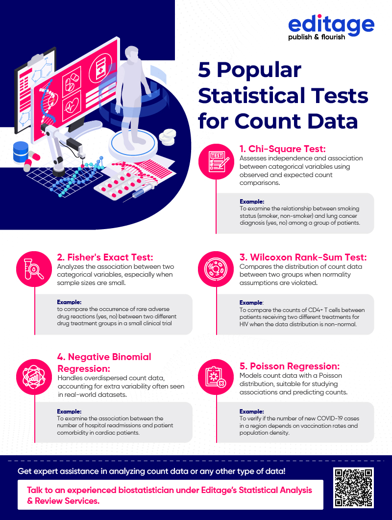
5 Popular statistical tests for count data_0.jpg